FAQ

To navigate, click topic in index to the right or search (Ctrl+f).

1 Setup project

1.1 Set up the overall project world

1.1.1 The scale of my map is wrong

The cellsize in the header of the imported .csv file is wrong. In dBSea you can use the Set world scale function to rescale your project. If the problem persists, open .csv in GIS editor or in another suitable software and set correct cellsize (maybe your cells are not square – see point 2).
Cells are not square, i.e. each cell is rectangular, extending further north-south than east-west (or the reverse). dBSea assumes square cells i.e. it expects that a map of dimensions X by Y data points is also X * cellsize by Y * cellsize in size. Use GIS software to re-sample map.

2 Sound Sources

2.1 Spectrum

2.1.1 What is Crest Factor?

The crest factor takes into account that spectrum levels are RMS levels and some peaks may have been “smoothed out” by this form of averaging. E.g. if crest factor is set 12 dB, SPLpeak will be calculated as 12 dB higher than the RMS value. Note that when using the NOAA weightings crest factor is not used directly as a measure of impulsivity.[1]

2.1.2 NOAA Classification of Impulsive and Non-Impulsive sounds

NOAA defines impulsive sounds as: [Sources that] produce sounds that are typically transient, brief (less than 1 second), broadband, and consist of high peak sound pressure with rapid rise time and rapid decay (ANSI 1986; NIOSH 1998; ANSI 2005).

And non-impulsive as: [Sources that] produce sounds that can be broadband, narrowband or tonal, brief or prolonged, continuous or intermittent and typically do not have a high peak sound pressure with rapid rise/decay time that impulsive sounds do (ANSI 1995; NIOSH 1998).

For sound classified as impulsive, NOAA publishes separate, lower thresholds (typically 15–20 dB lower for SEL_cum), reflecting the higher risk of injury from impulsive sound.[1] dBSea does not add anything to received levels; instead the predefined threshold sets in the database contain both impulsive and non-impulsive limits, and the impulsive limits are used automatically when the displayed level type is a time-series type (SEL_cum from a time series, SPL peak or peak-to-peak), while the non-impulsive limits are used for frequency-domain level types.

2.2 Multiple Sources

2.2.1 How do I add background noise levels?

Background levels cannot simply be added to dBSea scenarios; there is no ambient-noise input. Levels combine on an energy basis, so a background that sits well below the modelled source changes the total very little, and you can account for it by hand where it matters.

For example: if a ship is measured at 123 dB re 1 µPa (SPL) with background present, and the background alone is 120 dB, the background is 3 dB below the total and accounts for half of the mean-square pressure; the ship on its own is also 120 dB. In general, adding a background that is N dB below a source raises the total by 10·log₁₀(1 + 10^−N/10) dB: a background 3 dB below adds 1.8 dB, 10 dB below adds 0.4 dB, and 20 dB below adds 0.04 dB (Image 1). The result does not depend on the absolute level.

Image 1. Increase in the total level when background noise is combined with a source, as a function of how far the background sits below the source level.

2.3 Moving sources

2.3.1 How does the program interpret a moving source?

A moving source is modelled by making a series of discrete calculations along the moving path. The path waypoints and the number of intermediate calculation points are set by the user. More points give a better approximation, but increase computation time. No true line source calculation is possible, due to the varying bathymetry.

2.3.2 How does source speed influence my results?

The speed affects the source level by compensating for the amount of time spent at any given point. Notice that if two moving sources are present in the same scenario, the one of longer duration sets the time duration of the scenario. Hence a moving source of shorter duration will appear as having lower noise levels as it will be inactive for part of the scenario.

2.4 Piling and vertically extended sources

2.4.1 How do I model a piling source? Why is there no line source oriented in z?

Piling noise is dominated by low frequencies, which puts it firmly in the parabolic equation (PE) solver’s regime. The self-starter used by dBSea’s PE solver produces a vertical field that, at any range of practical interest, is essentially indistinguishable from the result you would get with a more sophisticated source model.

More sophisticated initialisations have been explored in the research literature, and we have tested some of these in-house and the differences in the received field are not significant for the kinds of distances and frequencies practising acousticians work at.

For practical use, place the source at the mid-depth of the pile. At low frequencies and typical project geometries the exact z position has relatively small impact on the field at distance.

2.4.2 How do I model a soft start (ramp-up) for piling?

A soft start gradually increases the hammer energy over the first part of a piling sequence, giving animals time to move away before full power is reached. How you account for it depends on what you are trying to produce:

Levels at a fixed receiver (probe or grid). The simplest approach is to fold the soft start into the Duty % parameter. Work out the effective duty cycle over the period of interest — accounting for the reduced energy during the ramp — and enter that single adjusted value. This avoids having to model each ramp step separately.
Animal exposure with the fleeing model. The fleeing calculation has direct support for soft-start parameters. Rather than approximating with duty cycle, you can enter the ramp profile and the model will apply the increasing source level over the soft-start period as animals respond — see § 2.6.1 and the Animal Movement page.

2.5 Time Series

2.5.1 How does dBSea handle surface ghosts?

The ray solver assumes a perfect reflection from the water surface. If the imported time series has no surface ghost (reflection), the Initial angles range Preferences → Advanced, Initial angles range should be set wide enough, so that some rays travel upward. The solver will create that ghost from the surface reflection. If the imported time series includes a surface ghost, angles should be set to exclude paths towards the surface.

2.5.2 What sample rate does my time series input need? Why are some bands showing a dash?

For a time-domain solve, the sample rate of the imported time series sets the highest frequency the data can represent. The Nyquist frequency (half the sample rate) must sit at least 5% above the upper edge of the highest band you want to solve for — otherwise that band cannot be resolved from the input.

Note that dBSea displays centre frequencies in the UI throughout the program (e.g. a “1 kHz” band is labelled by its centre). The Nyquist requirement applies to the upper edge of the band, which is above the centre frequency:

Octave bands: upper edge = centre × √2 ≈ 1.414 × centre
Third-octave bands: upper edge = centre × 2^1/6 ≈ 1.122 × centre

As quick rules of thumb, in terms of the centre frequency f_c of the highest band you want to solve for:

For octave bands, the input sample rate should be at least 3 × f_c.
For third-octave bands, the input sample rate should also be at least 3 × f_c: the band filter itself can be built from about 2.4 × f_c, but the solver skips any band whose centre frequency is above the sample rate divided by 2√2, so a band that shows a level in the import table may still be left out of the solve.

2.6 Animal exposure (fleeing model)

2.6.1 How does the fleeing model decide where the exclusion zone sits?

The fleeing model works on the solved sound field. Starting from the chosen initial position (normally the source), it sends a receiver straight outward along each radial slice of the project at the fleeing speed, reading the weighted broadband level from the solved grid every 10 seconds (a fixed step) and energy-summing those levels into a cumulative SEL.

In threshold mode, for each direction dBSea finds the smallest starting range from which an animal fleeing outward accumulates no more than the chosen SEL_cum threshold over the rest of its path. Where a soft start is defined, each step uses the source level in force at that moment in the ramp, so the animal’s early retreat is credited against the reduced levels it actually experienced.

The reported range is the worst case across all directions — that is, the direction in which the threshold is met furthest from the source. Because propagation is not the same in every direction (bathymetry, sound speed profile and source directivity all vary with bearing), the required starting range differs from angle to angle, and reporting the worst angle keeps the result protective in every direction. Note that the fleeing model reports a range and bearing in its own dialog; it does not draw the exclusion zone shown in the graphics area.

You can also fix the starting distance and read off the worst-case SEL, or define a custom path (waypoints with speeds) and read off the SEL accumulated along it.

For the controls, defaults and soft-start setup, see the Animal Movement page.

2.6.2 What source level should I enter for a fleeing calculation?

Whichever form is most convenient. Internally dBSea converts every source level input type to an equivalent continuous source level at 1 m, so entering an SEL over 1 second or a cumulative SEL over the full exposure (a 6-hour working day, say) will convert to the same internal level. There is no separate “fleeing model” input to prepare. The fleeing model then reads the solved field as sound pressure levels and energy-sums them over its 10 s steps with the scenario weighting applied, so the level type and assessment period chosen for display do not affect the result.

2.6.3 Is the fleeing model valid for impulsive sources such as piling or airguns?

Frequency-domain solves in dBSea always assume an equivalent continuous noise source. Where the true source is impulsive, this remains a well-justified assumption as long as the repeating impulse window (say 10 seconds between impulses) is short compared to the total fleeing time. Put another way: the animal swims slowly enough that within any one impulse window it stays inside a region of approximately constant received level.

2.7 Impulsive sources and level scaling (SEL_ss, SEL_cum)

2.7.1 How do I enter a single-strike SEL (SEL_ss)? Do I need to set a window or duty cycle for it?

A single-strike SEL — the energy of one pile strike, one airgun firing, or any other single impulsive event — is not a time-dependent input, and this is where it differs from dBSea’s other frequency-domain source levels.

For a continuous source, dBSea assumes the entered level holds constant across the whole assessment window, so the window length matters: a longer window means more energy. An impulse is the opposite. All the energy of the event is already captured within whatever measurement window produced the SEL_ss figure. Extending that window would capture nothing more, because there is nothing left outside it. The value is simply “the energy of one event”, and the length of the window it was measured over is irrelevant.

So you do not need to — and should not — reach for the Duty % to represent a single strike. dBSea has no separate single-strike input type: enter the SEL_ss with the Sound exposure level level type and make the Assessment period for source (s) equal to the Assessment period for results (see § 2.7.2), and the value you read out is the value you put in. The accumulation to a full exposure is handled separately (see § 2.7.3).

2.7.2 Which input and output metric should I use to avoid scaling surprises?

The confusion people most often hit is not really about SEL_ss itself — it is about the fact that dBSea applies a level scaling twice: once on input (converting the level you enter into its internal representation over the assessment period) and again on output (converting the internal level back to the metric you have chosen to display, over the assessment period).

The simplest way to stay in control is to use SEL_cum on both input and output, with the same assessment period on each side. One second is the natural choice, but the actual value does not matter — what matters is that it is the same for input and output. When the two assessment periods match, the input and output scaling cancel exactly, and the level you read out is the level you put in, with no hidden conversion applied. This removes the guesswork and is the recommended recipe whenever you are working with impulsive sources.

2.7.3 I have a known number of strikes, how do I get to a cumulative SEL?

Use the Count parameter. In a typical assessment the engineer knows the total number of impulse events — for example the hammer strikes in a piling sequence, or the shots in an airgun run. Set Count to that number, and dBSea energy-sums the single-event SEL up to the total accumulated SEL. In this scenario the meaningful output metric is typically SEL_cum.

Count, not Duty %, is the mechanism that turns one event into many. Duty % should generally stay at 100% for a strike-counted impulsive source. It has a legitimate role only if something in the impulse sequence genuinely justifies it — for instance a gap between activity periods within the assessment window — and that is left to the user’s discretion.

3 Solver and Frequencies

3.1 Solver choice

3.1.1 Should I use the 2D or the 3D solvers?

Use the 3D solvers (dBSeaPE 3D and dBSeaRay 3D) for most work. They model propagation in all directions, so sound reaches areas that have no direct line of sight to the source, such as behind islands and headlands.

The 2D solvers (dBSeaPE and dBSeaRay) calculate levels in straight radial slices out from the source. Areas without line of sight will typically show no levels, or levels that are too low, depending on the local bathymetry. They remain available for older projects and for simple, open-water scenarios where their speed is useful. If you do use a 2D solver in a scenario with many small islands, untick Stop marching solution upon reaching land in Preferences → Advanced.

3.1.2 I have a `Solver found no modes at location` error, what does this mean?

This message comes from the normal modes solver (dBSeaModes) used in older versions. For low frequencies mode ‘shapes’ are very large and in shallow water that can lead to a situation where the root finder finds no solution. dBSea v3 no longer offers the modes solver; projects that used it are switched to dBSeaPE when opened, which does not have this limitation.

3.2 Frequency Selection

3.2.1 What should my crossover frequency be?

This depends on your scenario. In deep water the crossover is less important and can be set low, letting the ray tracer handle most frequencies. In shallow water, a crossover around 500 Hz to 1 kHz is typical. See General Modelling Tips § 2.1 for detailed guidance by scenario type.

3.3 Solvers

3.3.1 Which solvers support directivity?

As of v3.0.11, directivity is supported by dBSeaRay (3D and 2D) and dBSeaPE (3D and 2D). The simple geometric spreading solvers (10 log, 20 log) do not support directivity.

3.3.2 How accurate are the solvers?

There’s no simple answer to this, but all solvers are tested and validated against benchmark solvers from Computational Ocean Acoustics (Jensen 2011). The dBSea solvers will give slightly higher levels when the Levels must decrease with distance is ticked and the Radial smoothing factor is different from zero. We continuously validate and update the solvers as we obtain more real world data.

3.3.3 Why do I get no values close to the source when using the ray tracer?

This is most likely caused by having the angle of the ray tracer set too narrow. Open Preferences → Advanced and adjust Initial angles range and Initial step size.

3.3.4 Will a large number of seabed layers, location properties in the properties map, or in a sound speed profile slow down my solve?

In most cases, no — the effect is negligible. Properties such as the sound speed profile and seabed details are interpolated on the fly during the solve, and this interpolation is very cheap compared to the propagation calculations the solvers perform. You can specify detailed profiles with many points, and many locations in the properties map without worrying about a significant impact on solve time.

4 Overall Sound Levels

4.1 Output level display and conversion

4.1.1 Do I need to re-solve when changing the displayed level type?

For frequency-domain solves, switching between Sound pressure level (SPL) and Sound exposure level (SEL_cum) needs no re-solve: results are stored as SPL and converted on the fly using the Assessment period for results, so you can change the level type in Preferences → Sound levels display and see the updated results immediately. This also holds for scenarios with moving sources.

Two cases do require a re-solve, and the Preferences page warns about them:

Changing to or from Max sound pressure level (the crest-factor peak estimate), because moving-source positions and multiple sources are combined as a maximum for this type rather than energy-summed.
Any change between the time-series level types: Sound exposure level, Peak sound pressure level and Peak to peak sound pressure level. SEL is stored per band, while peak and peak-to-peak are each stored as a single broadband number per grid point and the waveform is discarded, so none of the three can be derived from another after the solve.

All other conversions — including between SPL and L_E/SEL for non-time-series results — are performed on the fly without a re-solve.

4.2 Change Limits

4.2.1 Exclusion zone and sound level contours are not equal

The exclusion zone is calculated radially around the source and is made to give a contiguous area. The user also has the option of choosing a different radial smoothing factor for the exclusion zone.

4.2.2 I’ve ticked the `Show exclusion zone` box, but no exclusion zone appears/exclusion zone looks very irregular.

Check that you have selected a criterion in either the Exclusion zone level (dB) box or the threshold dropdown next to it (predefined thresholds from the database).
The exclusion zone is partly based on the amount of radial slices used Setup project → Radial slices. Fewer than 4 slices are refused with the message Too few slices to show exclusion zone. Also keep in mind that using very few radial slices in a complex scenario, will severely impact accuracy.

5 Water properties and Sound speed profile

5.1 Sound speed profile

5.1.1 I get a very irregular sound field.

Depending on the scenario, very sudden changes in sound speed can cause the model to output unexpected results. Try to make the sound speed profile more smooth by adding more points in the Sound speed profile window.

5.2 Attenuation Profile

5.2.1 Why do results remain the same after I change the temperature of the water?

Frequency specific attenuation is only relevant at high frequencies (>10 kHz), so often the soundscape (and the results) will be dominated by lower frequencies, whose propagation is not/barely affected by temperature. The absorption graph (accessed via the tab buttons next to the temperature and salinity input) shows the current absorption curve.

5.2.2 How does temperature and salinity affect propagation?

Under 10 kHz frequency-specific attenuation is less than 1 dB/km, and salinity and temperature only account for a very little part of this.

Try National Physics Laboratory’s calculator.

6 Graphics Window

6.1 Land is not land coloured

In ESRI Ascii grid .asc files, areas may be given as NO_DATA, meaning there is no measured height or depth at that point. dBSea treats this differently than land. You can set the display colour for NO_DATA areas on the preferences form.

6.2 The Bathymetry is inverted/upside down

dBSea uses the convention that positive values are depths (below the surface) and negative values are heights (above the surface).

Some common bathymetry datasets use the opposite z-axis sign convention — for example GEBCO, where depths are negative and elevations positive. When data like this is imported without adjustment, the bathymetry will appear inverted: the sea floor reads as terrain and vice versa.

Two ways to fix this in dBSea:

Tools → Swap heights and depths (this does not change the bathymetry file, but will be stored in the dBSea project file)
Open CSV-editor. Tools → Launch CSV Editor. Import your bathymetry, press Translate, choose Reverse heights and depths. Export current selection. (This stores a new bathymetry file with swapped heights and depths).

7 Exporting

7.1 The `Export to GIF` returns an error

When using the gif-tool, dBSea has to save and access values at all positions along any given track. On some computers this intense use of memory can lead to an error. To resolve this, try to either free up some RAM-space (by closing other applications) or reduce some parameter of your model (size of calculation grid, number of frequencies solved for, dB-resolution or showing fewer depth slices).

8 CSV Editor

8.1 Bathymetry import

8.1.1 What coordinate system does the CSV Editor use?

CSV Editor and dBSea both work in metres easting/northing internally.

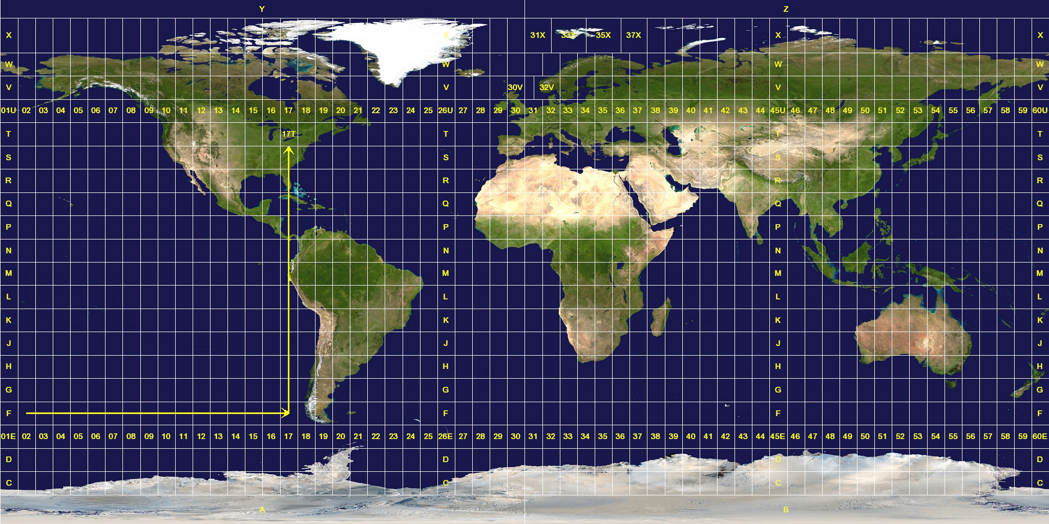
ESRI Ascii Grid files have a header that specifies the location and size of the data. This can be given in metres, or in degrees latitude/longitude. dBSea will guess that degrees are used if the values are all less than ±360°. If you confirm that the coordinates are in degrees, dBSea will, where possible, convert to metres using a UTM zone, with the zone chosen based on the middle of the import area.

For more on how dBSea handles coordinate systems, UTM zones, and lat-long conversion, see § 9 Coordinate Systems and UTM Zones.

9 Coordinate Systems and UTM Zones

9.1 How dBSea handles coordinates

9.1.1 What coordinate system does dBSea work in?

dBSea works in whatever coordinate system your bathymetry is supplied in. Internally it uses metres easting/northing (a projected, metre-based system), and on import it will convert your data to easting/northing where possible — including from latitude/longitude.

How the coordinate settings are established depends on your input:

Geotagged easting–northing input. If your bathymetry is appropriately geotagged, dBSea retains those coordinate settings (offsets and UTM zone) as-is.
Latitude/longitude input. dBSea can import lat-long data and, where possible, will automatically convert it to easting–northing on input and assign a UTM zone, choosing the zone from the middle of the import area. Note that some formats (e.g. ESRI Ascii Grid) do not unambiguously state their coordinate system, so dBSea relies on a heuristic to detect lat-long — it guesses that degrees are in use when all values are within ±360°. Where the coordinate system cannot be determined this way, dBSea may not attempt a conversion, and you can set the offsets and UTM zone manually instead. See also § 9.1.3 on degree-input skew.
Untagged input. If the input is not geotagged, the easting and northing offsets are initialised to 0. You can update them manually if you need real-world positions.

You can also set everything manually:

Easting/northing offsets — these point at the bottom-left (south-west) corner of the project area.
UTM zone — set the zone directly if the automatic choice is not what you want.

See the Coordinates page for how dBSea designates UTM zones.

9.1.2 What’s the recommended workflow for getting bathymetry into the right coordinate system?

It is recommended that you use external GIS software (QGIS, ArcGIS, etc.) to get your bathymetry into a UTM-zone, geotagged format that works for dBSea. Doing the projection in GIS up front has a further benefit: dBSea will then export results in the same coordinate system, so the output can be imported directly back into your GIS software for mapping and reporting.

For simple position conversions — for example, placing individual sources and probes when you have their coordinates in a different system — dBSea provides a built-in latitude/longitude ↔ UTM converter. This is handy for one-off point conversions; for anything involving the bathymetry grid itself, GIS software has far more capability and should be preferred.

Bathymetry import is handled via the CSV Editor.

9.1.3 Degree-based input and UTM zone skew

Files where the locations are given in degrees are necessarily skewed due to the curvature of the Earth. These effects are greater closer to the poles, and for large areas. If the skewing is too great, conversion in a GIS package to easting/northing in metres is recommended.

Note that the official UTM zones around Skagerrak (Denmark/Norway) and Svalbard (Norway) are skewed (UTM Zones Map). dBSea does not take these irregularities into account, so if you work in any of these zones, check and manually correct the northing/easting.

10 Memory

10.1 Memory usage

10.1.1 I’m running out of memory

Storing all the calculated sound levels takes a large amount of memory. This can be reduced by lowering the number of source slices, range points, depth points, frequencies, and x and y output grid points.

You can also use our model size calculator. Simply, update the numbers in the input section.

10.1.2 Improved memory handling (v3.0.15+)

Version 3.0.15 introduced significant improvements to how dBSea handles memory for large models. Models that previously required very large amounts of RAM can now run on machines with more modest memory.

If you are running out of memory on v3.0.15 or later, check that you have adequate free disk space on the drive where dBSea stores its temporary files, as the newer versions make use of disk space to reduce RAM requirements.

10.1.3 Reduced peak memory usage during solves (v3.0.21+)

Versions 3.0.21 to 3.0.23 substantially reduce the peak memory used while a solve is running: 3.0.21 reduced memory pressure for all PE solves, 3.0.22 reduced the memory used by the levels cache, and 3.0.23 bounds memory growth in the 3D ray solver. If you have been seeing out-of-memory or heap space errors during solves, upgrade to the current version first.

11 Miscellaneous

11.1 Does dBSea work in fresh water?

Yes, simply set the salinity to 0.

11.2 Can I run dBSea in batch mode?

Yes, in several ways. A command-line script mode (-s <script file>) runs a text script with commands to load a project or bathymetry, solve, and write levels and probe results; run dBSea with -h for the command list. Within a session, Tools → Python interface offers a Python scripting console, and licences with the API feature can start a local HTTP API (also from the command line with -a <port>, v3.0.18+). For comparing parameter variations within one project, use the Scenarios tab.

11.3 dBSea on Linux and macOS

dBSea v3 is available for Linux (Debian/Ubuntu) and macOS. Contact the dBSea team for details. Wine is no longer required.

12 Terms and abbreviations

Batch mode: Terminology describing the process of applying the same algorithm to multiple files.
ESRI ASCII grid: Plain-text raster format with a short header (ncols, nrows, cellsize, NODATA value) followed by the gridded values.
Multi-Threading: Running several processes in parallel.
RMS: Root Mean Square, the effective (time-averaged) amplitude of a pressure signal; SPL is based on it.

13 References

NOAA. Technical Guidance for Assessing the Effects of Anthropogenic Sound on Marine Mammal Hearing. NOAA Technical Memorandum NMFS-OPR-55, 2016.
Jensen, F. B., Kuperman, W. A., Porter, M. B., & Schmidt, H. Computational Ocean Acoustics, 2nd ed. Springer, 2011.